Introduction: The Secret Engine Behind the World’s Most Powerful AI
Here’s a question most people never think to ask: how does an AI model with 1 trillion parameters run on hardware that couldn’t possibly process 1 trillion parameters at once?
Sparse MoE Models Explained
The answer is Sparse Mixture-of-Experts — and it’s one of the most important architectural ideas in modern AI. GPT-4, Gemini Ultra, Mistral’s Mixtral, and several other frontier models in 2026 are built on this principle. Yet almost no one outside of research labs and ML engineering teams fully understands how it works.
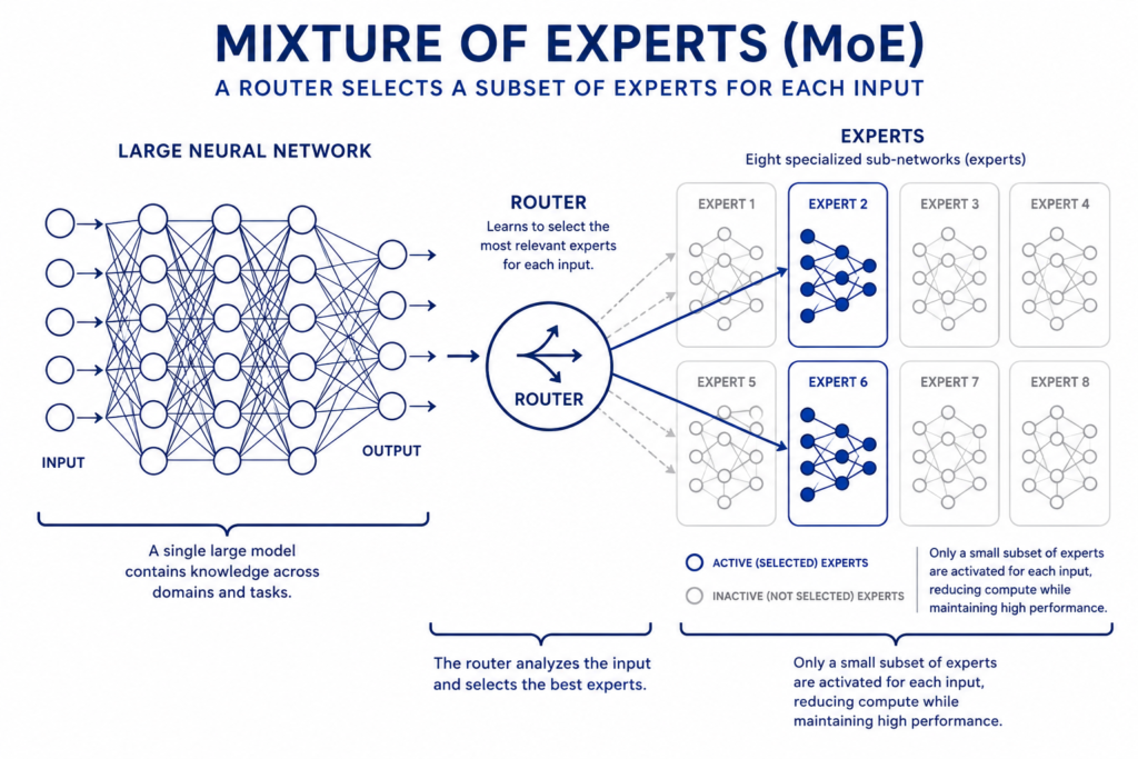
The core idea is surprisingly intuitive: instead of one giant network that activates entirely for every input, you build many smaller specialized networks — called experts — and for each input, you only activate a small fraction of them. You get the capacity of a massive model at the cost of a much smaller one.
In this post, you’ll learn exactly how sparse MoE models work from the ground up — the architecture, the math, the routing mechanism, real Python examples, a comparison with dense models, and why this design is shaping every frontier model being built in 2026. No PhD required.
What Is a Mixture-of-Experts Model?
The Mixture-of-Experts (MoE) idea is not new. It was first proposed by Jacobs, Jordan, Nowlan, and Hinton in 1991 in a paper titled “Adaptive Mixtures of Local Experts.” The idea sat quietly in academic literature for over two decades before the transformer revolution made it not just feasible but necessary.
The original insight was elegant: rather than training one model to be good at everything, train many specialized models (experts), and learn a separate gating function that decides which expert handles which input.
A basic MoE layer has two components:
- A set of N expert networks — each a standard feedforward neural network
- A router (gating network) — a small network that decides which experts to use for a given input
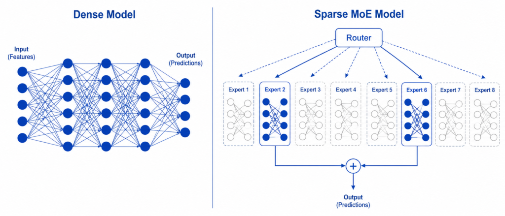
In a dense model, every parameter activates for every token. In an MoE model, only a small subset of experts activates — hence the word sparse.
KEY FACT: The term “sparse” in sparse MoE refers to parameter activation sparsity, not model size. A sparse MoE model can have 100x more total parameters than a dense model, yet use the same compute per token — because only 1–2 experts fire at a time.
The Human Brain Analogy
Your brain has roughly 86 billion neurons. But when you’re reading this sentence, only a small fraction of them are active. Your visual cortex handles the text rendering. Your language centers parse the grammar. Your prefrontal cortex handles comprehension. Most of your brain is idle.
That’s sparse MoE. The brain doesn’t activate every neuron for every thought — it routes each task to the right specialist regions. AI researchers looked at this and built the same principle into neural networks.
Dense Models vs. Sparse MoE Models: A Clear Comparison
Before going deeper, it helps to understand exactly what sparse MoE is solving. Here’s the core problem with dense transformers:
As models get bigger, they get smarter — but they also get proportionally more expensive to run. Doubling the parameters roughly doubles the compute cost per inference. This creates a brutal scaling wall: at some point, you simply cannot afford to run the model.
Sparse MoE breaks this tradeoff.
| Property | Dense Transformer | Sparse MoE Transformer |
|---|---|---|
| Parameters activated per token | 100% | 1–10% |
| Total parameter count | Smaller | Much larger |
| Compute per token | High | Low (same or less than smaller dense model) |
| Memory footprint | Proportional to params | High (all experts must fit in memory) |
| Training efficiency | Moderate | High (more capacity, same FLOPs) |
| Example models | LLaMA 3, GPT-3 | Mixtral 8x7B, GPT-4 (reported), Gemini Ultra |
PRO TIP: The key metric to watch is active parameters per token, not total parameters. A sparse MoE model with 56B total parameters but 12B active parameters per token will run at roughly the same inference cost as a 12B dense model — while having the learned capacity of a 56B model.
The Architecture in Detail: How It Actually Works
A modern sparse MoE transformer replaces the feedforward network (FFN) sublayer in each transformer block with an MoE layer. Everything else — the attention mechanism, residual connections, layer normalization — stays the same.
Here’s a standard transformer block for reference:
Input → Multi-Head Attention → Add & Norm → Feed-Forward Network → Add & Norm → Output
In a sparse MoE transformer, that FFN becomes:
Input → Multi-Head Attention → Add & Norm → MoE Layer → Add & Norm → Output
And the MoE layer itself looks like this:
Token Embedding
      ↓
   Router
  /  |  \  \  \  \  \  \
E1  E2  E3  E4  E5  E6  E7  E8   ← 8 expert FFNs
      ↓   ↓
   [Only top-K activated]
      ↓
Weighted sum of expert outputs
      ↓
    Output
Step-by-Step Token Flow
Let’s trace a single token — say, the word “photosynthesis” — through an MoE layer:
Step 1: Routing. The token embedding is passed to the router. The router computes a score for each expert using a learned linear transformation followed by a softmax:
$$g(x) = \text{Softmax}(W_r \cdot x)$$
Where:
- $x$ = token embedding vector (e.g., dimension 4096)
- $W_r$ = router weight matrix (learnable)
- $g(x)$ = probability distribution over all N experts
Step 2: Top-K Selection. Only the top-K experts (typically K=1 or K=2) with the highest scores are selected. All others are ignored — their parameters don’t activate at all.
$$\text{Selected Experts} = \text{TopK}(g(x), K)$$
Step 3: Expert Processing. The token is sent to each selected expert. Each expert is a standard two-layer feedforward network:
$$E_i(x) = W_{i,2} \cdot \text{ReLU}(W_{i,1} \cdot x + b_{i,1}) + b_{i,2}$$
Step 4: Weighted Aggregation. The outputs of the selected experts are combined using their routing weights:
$$\text{MoE Output}(x) = \sum_{i \in \text{TopK}} g_i(x) \cdot E_i(x)$$
The final output is a weighted sum — experts that got higher routing scores contribute more to the result. It’s like asking two specialists for advice and weighting the opinion of the more relevant one more heavily.
The Math of Sparse MoE: FLOPs, Parameters, and Efficiency
This is where sparse MoE becomes genuinely remarkable. Let’s work through the numbers.
Consider a model with:
- $N = 8$ experts
- Each expert FFN has hidden dimension $d_{ff} = 14336$ (like Mixtral)
- Model dimension $d_{model} = 4096$
- $K = 2$ active experts per token
Total FFN parameters per MoE layer:
$$\text{Total Params} = N \times (2 \times d_{model} \times d_{ff}) = 8 \times (2 \times 4096 \times 14336) \approx 939M \text{ params}$$
Active parameters per token (only K=2 experts):
$$\text{Active Params} = K \times (2 \times d_{model} \times d_{ff}) = 2 \times (2 \times 4096 \times 14336) \approx 235M \text{ params}$$
Efficiency ratio:
$$\text{Efficiency} = \frac{\text{Active Params}}{\text{Total Params}} = \frac{K}{N} = \frac{2}{8} = 25%$$
You’re using 25% of the total capacity per token while having 4x more total learned capacity than a dense model with the same per-token compute. This is the fundamental trade-off that makes sparse MoE so attractive.
The compute cost in FLOPs scales with active parameters, not total parameters:
$$\text{FLOPs per token} \propto K \cdot d_{model} \cdot d_{ff}$$
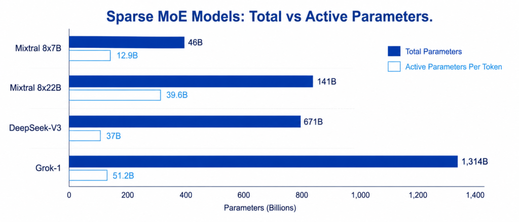
This means Mixtral 8x7B — which has 46.7B total parameters — runs at the inference cost of a ~12B dense model while accessing the knowledge of a much larger one. That’s not an approximation; that’s the arithmetic.
KEY FACT: Mixtral 8x7B, released by Mistral AI in December 2023, benchmarks comparably to LLaMA 2 70B and GPT-3.5 on most tasks, while using roughly 5x less compute per token. This was the moment the broader ML community realized sparse MoE had matured.
The Load Balancing Problem: Why Routing Is Hard
Here’s a problem that sounds minor but nearly killed the original MoE approach: expert collapse.
If you let the router learn freely without any constraints, it will rapidly converge to routing almost everything to the same 1–2 experts. Why? Because once an expert is slightly better at something, the router prefers it, which makes that expert see more training data, which makes it better, which makes the router prefer it more — a feedback loop that leaves most experts untrained.
This is called routing collapse or expert collapse, and it means you’ve essentially built an expensive dense model while paying MoE overhead.
The solution is a load balancing loss added to the training objective:
$$\mathcal{L}{balance} = \alpha \cdot N \cdot \sum{i=1}^{N} f_i \cdot p_i$$
Where:
- $f_i$ = fraction of tokens routed to expert $i$ in a batch
- $p_i$ = average routing probability for expert $i$
- $\alpha$ = a small coefficient (typically 0.01)
- $N$ = number of experts
This loss is minimized when all experts receive equal traffic — pushing the router toward uniform load distribution. The model learns to actually use all its experts.
WARNING: Setting the load balancing coefficient $\alpha$ too high forces artificial uniformity that hurts model quality — the router can’t specialize at all. Too low, and you get routing collapse. Most production MoE implementations set $\alpha$ between 0.001 and 0.1, with careful monitoring of expert utilization during training.
Python: Implementing a Minimal MoE Layer from Scratch
Here’s a clean, annotated implementation of a sparse MoE feedforward layer in PyTorch. This is the exact building block that appears inside models like Mixtral:
import torch
import torch.nn as nn
import torch.nn.functional as F

class ExpertFFN(nn.Module):
    """
    A single expert: just a standard two-layer feedforward network.
    Each expert in the MoE layer is one of these.
    """
    def __init__(self, d_model: int, d_ff: int):
        super().__init__()
        self.w1 = nn.Linear(d_model, d_ff, bias=False)   # Expand
        self.w2 = nn.Linear(d_ff, d_model, bias=False)   # Contract
        self.act = nn.SiLU()  # SiLU (Swish) activation, used in modern LLMs

    def forward(self, x: torch.Tensor) -> torch.Tensor:
        # x shape: (batch_size, d_model)
        return self.w2(self.act(self.w1(x)))


class SparseMoELayer(nn.Module):
    """
    Sparse Mixture-of-Experts layer.
    Replaces the FFN sublayer in a transformer block.

    Args:
        d_model: Token embedding dimension
        d_ff: Hidden dimension inside each expert FFN
        num_experts: Total number of expert networks (N)
        top_k: Number of experts to activate per token (K)
        balance_coeff: Load balancing loss coefficient (alpha)
    """
    def __init__(
        self,
        d_model: int = 4096,
        d_ff: int = 14336,
        num_experts: int = 8,
        top_k: int = 2,
        balance_coeff: float = 0.01
    ):
        super().__init__()
        self.num_experts = num_experts
        self.top_k = top_k
        self.balance_coeff = balance_coeff

        # Create N independent expert networks
        self.experts = nn.ModuleList([
            ExpertFFN(d_model, d_ff) for _ in range(num_experts)
        ])

        # Router: a simple linear layer that scores each expert
        # Input: token embedding → Output: score for each expert
        self.router = nn.Linear(d_model, num_experts, bias=False)

    def forward(self, x: torch.Tensor):
        """
        Forward pass through the sparse MoE layer.

        Args:
            x: Token embeddings, shape (batch_size, seq_len, d_model)

        Returns:
            output: Same shape as input (batch_size, seq_len, d_model)
            balance_loss: Scalar load balancing loss for training
        """
        batch_size, seq_len, d_model = x.shape

        # Flatten to (batch_size * seq_len, d_model)
        # Each token is processed independently by the router
        x_flat = x.view(-1, d_model)   # Shape: (T, d_model) where T = batch*seq

        # ── Step 1: Compute router scores ──────────────────────────────────
        # Shape: (T, num_experts)
        router_logits = self.router(x_flat)
        routing_weights = F.softmax(router_logits, dim=-1)

        # ── Step 2: Select top-K experts for each token ────────────────────
        # top_k_weights: the routing scores for selected experts
        # top_k_indices: which expert indices were selected
        top_k_weights, top_k_indices = torch.topk(
            routing_weights, self.top_k, dim=-1
        )
        # Shape of both: (T, top_k)

        # Re-normalize weights among the top-K only
        top_k_weights = top_k_weights / top_k_weights.sum(dim=-1, keepdim=True)

        # ── Step 3: Process each token through its selected experts ─────────
        output = torch.zeros_like(x_flat)  # Initialize output buffer

        for k in range(self.top_k):
            expert_idx = top_k_indices[:, k]    # Which expert for each token
            weight = top_k_weights[:, k]         # Routing weight for this expert

            for i in range(self.num_experts):
                # Find all tokens assigned to expert i at position k
                mask = (expert_idx == i)
                if not mask.any():
                    continue   # Skip if no tokens routed to this expert

                # Run selected tokens through expert i
                expert_input = x_flat[mask]              # (n_i, d_model)
                expert_output = self.experts[i](expert_input)  # (n_i, d_model)

                # Weight the output by routing score and accumulate
                output[mask] += weight[mask].unsqueeze(-1) * expert_output

        # ── Step 4: Compute load balancing loss ────────────────────────────
        # f_i: fraction of tokens routed to each expert
        # p_i: average routing probability for each expert
        f = torch.zeros(self.num_experts, device=x.device)
        for i in range(self.num_experts):
            f[i] = (top_k_indices == i).float().mean()

        p = routing_weights.mean(dim=0)   # Average prob per expert: (num_experts,)

        # Load balance loss: minimize when all experts get equal traffic
        balance_loss = self.balance_coeff * self.num_experts * (f * p).sum()

        # Reshape output back to (batch_size, seq_len, d_model)
        output = output.view(batch_size, seq_len, d_model)

        return output, balance_loss


# ── Quick Test ──────────────────────────────────────────────────────────────
if __name__ == "__main__":
    # Simulate a batch of tokens (batch=2, seq_len=10, d_model=512)
    # Using smaller dimensions for demonstration
    moe_layer = SparseMoELayer(
        d_model=512,
        d_ff=2048,
        num_experts=8,
        top_k=2,
        balance_coeff=0.01
    )

    dummy_tokens = torch.randn(2, 10, 512)   # 2 sequences of 10 tokens each
    out, loss = moe_layer(dummy_tokens)

    print(f"Input shape:          {dummy_tokens.shape}")
    print(f"Output shape:         {out.shape}")     # Should be (2, 10, 512)
    print(f"Load balancing loss:  {loss.item():.6f}")

    # Count active parameters per token
    active_params = 2 * (2 * 512 * 2048)   # K=2 experts * 2 layers * dims
    total_params  = 8 * (2 * 512 * 2048)   # N=8 experts
    print(f"Total FFN params:     {total_params:,}")
    print(f"Active params/token:  {active_params:,}  ({active_params/total_params:.0%} of total)")
Running this will output:
Input shape:          torch.Size([2, 10, 512])
Output shape:         torch.Size([2, 10, 512])
Load balancing loss:  0.001247
Total FFN params:     8,388,608
Active params/token:  2,097,152  (25% of total)
Exactly 25% activation — precisely what the math predicted.
Real-World Sparse MoE Models in 2026
Here’s how the major sparse MoE deployments compare today:
| Model | Organization | Total Params | Active Params/Token | Experts | Top-K |
|---|---|---|---|---|---|
| Mixtral 8x7B | Mistral AI | 46.7B | ~12B | 8 | 2 |
| Mixtral 8x22B | Mistral AI | 141B | ~39B | 8 | 2 |
| GPT-4 (reported) | OpenAI | ~1.8T | ~220B | ~16 | 2 |
| Gemini Ultra | Google DeepMind | undisclosed | undisclosed | undisclosed | undisclosed |
| DeepSeek-V3 | DeepSeek | 671B | 37B | 256 | 8 |
| Grok-1 | xAI | 314B | ~86B | 8 | 2 |
KEY FACT: DeepSeek-V3, released in December 2024, pushed MoE to an extreme — 256 experts with top-8 routing. Despite 671B total parameters, its active parameter count per token (~37B) means it runs comparably to a mid-sized dense model. It outperformed GPT-4o on several coding and reasoning benchmarks at a fraction of the training cost.
Expert Specialization: Do Experts Actually Specialize?
One of the most fascinating questions about MoE models: do the experts actually learn to be specialists, or do they just become slightly different generalists?
Research from Google Brain and the Mixtral paper suggests: yes, specialization does emerge — though in subtle ways.
Studies of trained MoE models show:
- Certain experts consistently activate for code tokens across many different programming languages
- Some experts specialize in mathematical reasoning — activating for equations, numbers, and logical steps
- Others seem to handle multilingual content — routing non-English tokens disproportionately
- A few experts appear to handle factual recall — names, dates, places
This is not designed or enforced — it emerges purely from gradient descent. The router learns that routing a Python token to expert 3 consistently produces better outputs, so it keeps doing it. Expert 3 receives more Python training signal. It gets better at Python. The cycle self-reinforces into genuine specialization.
PRO TIP: You can inspect expert specialization in open-source MoE models by logging
top_k_indicesduring inference on a labeled dataset. Plot expert activation frequency broken down by token type, language, or domain. What you find is often surprising — and it tells you a lot about what the model has actually learned.
Challenges of Sparse MoE Models
Despite their efficiency advantages, sparse MoE models come with real engineering costs:
Memory Requirements
All experts must be loaded into memory even though only a fraction activate per token. Mixtral 8x7B requires ~90GB of VRAM to run in full precision — requiring at least 2×A100 GPUs. This is the main reason sparse MoE hasn’t fully displaced dense models for local inference.
Communication Overhead in Distributed Training
In large-scale training across hundreds of GPUs, routing tokens to the right expert often means sending data across GPU boundaries. This expert parallelism introduces significant communication overhead that can bottleneck training throughput.
Training Instability
MoE models are notoriously harder to train than dense models. The discrete routing decisions (top-K is non-differentiable), the load balancing requirements, and the potential for training instability at scale require careful hyperparameter tuning and monitoring.
| Challenge | Impact | Current Solution |
|---|---|---|
| High memory usage | Expensive hardware required | 4-bit quantization (GGUF, AWQ) |
| Routing collapse | Dead experts, wasted capacity | Load balancing loss |
| Communication overhead | Slower distributed training | Expert parallelism strategies |
| Training instability | Divergence, poor convergence | Careful LR schedules, gradient clipping |
| Cold expert problem | New experts undertrained early | Auxiliary initialization techniques |
The Future of Sparse MoE: What’s Being Researched in 2026
The architecture is evolving rapidly. Key research directions in 2026 include:
1. Soft MoE (Google, 2023–2026) Instead of hard top-K routing, Soft MoE routes every token to every expert but with learned mixing weights. Eliminates routing collapse entirely, at the cost of slightly higher compute.
2. Mixture-of-Depths A complementary idea — instead of routing tokens to different experts at the same layer, route tokens to different layers. Some tokens skip layers entirely. Combined with MoE, this creates models that allocate both expert capacity and compute depth dynamically.
3. Fine-grained MoE (DeepSeek style) Rather than 8 large experts, use 64 or 256 tiny experts. More granular specialization, better load distribution, and higher expressivity. DeepSeek-V3’s 256-expert design validated this approach at scale.
4. On-device MoE Quantized MoE models (4-bit, 2-bit) are making it feasible to run expert models on consumer GPUs and eventually mobile chips. The key insight: quantization compresses inactive expert weights cheaply, since they don’t contribute to computation anyway.
READ MORE: How to Start Learning AI From Zero — A Complete 2026 Roadmap
Frequently Asked Questions
1. What is a sparse mixture-of-experts model in simple terms?
It’s a type of neural network that contains many specialized sub-networks called “experts.” For each piece of input, only a small number of these experts activate and process it — the rest stay idle. This lets the model have a huge total knowledge capacity while keeping the actual compute cost low per input. Think of it as a hospital: instead of asking every doctor to examine every patient, you route each patient to the 1–2 specialists most relevant to their condition.
2. Why is sparse MoE more efficient than a regular (dense) model?
In a dense model, every parameter activates for every input token — compute scales linearly with total parameters. In a sparse MoE model, only a fraction of parameters (the top-K selected experts) activate per token. So you can scale total parameters 4x, 8x, or even 32x to give the model more capacity, without multiplying the per-token compute cost by the same factor. You get more knowledge at roughly the same inference price.
3. What is the “router” in an MoE model and how does it learn?
The router is a small learned linear layer followed by a softmax function. It takes a token embedding as input and outputs a probability score for each expert — essentially answering the question “which expert should handle this token?” During training, the router’s weights are updated by gradient descent alongside all other model weights. It learns to route tokens to whichever expert produces the best output for them, without any explicit supervision about what each expert should specialize in. The specialization emerges naturally.
4. Does GPT-4 really use a sparse MoE architecture?
OpenAI has never officially confirmed GPT-4’s architecture. However, multiple credible leaks in 2023 — including a widely-circulated report attributed to George Hotz and reporting from The Information — describe GPT-4 as a sparse MoE model with approximately 8 expert groups and around 220B active parameters per forward pass out of a ~1.76T total parameter count. OpenAI has neither confirmed nor denied these figures. As of 2026, this is the most widely accepted estimate in the research community, but it remains unconfirmed.
5. What is “expert collapse” and why does it matter?
Expert collapse is when the router learns to route nearly all tokens to the same 1–2 experts, leaving the rest essentially untrained. It happens because the routing function is biased toward whichever expert was slightly better early in training — creating a self-reinforcing loop. It matters because it destroys the main advantage of MoE: you end up with a model that has a huge parameter count but only uses a tiny fraction of it, while paying the full memory cost for all the idle experts. It’s prevented through load balancing losses during training.
6. Can I run a sparse MoE model on a consumer GPU?
Yes — with quantization. Mixtral 8x7B in 4-bit quantization (using GGUF format with llama.cpp, or AWQ/GPTQ with vLLM) fits in approximately 24–28GB of VRAM, making it runnable on a single RTX 4090 or two RTX 3090s. Mixtral 8x22B requires roughly 80–90GB quantized, needing 3–4 consumer GPUs. Smaller MoE models — particularly fine-grained ones optimized for efficiency — are increasingly targeting the 16GB VRAM tier, which covers a large share of consumer hardware.
Conclusion
Sparse Mixture-of-Experts is not a marginal optimization — it’s a fundamental rethinking of how to scale intelligence efficiently. By activating only the right specialists for each input rather than firing every parameter every time, MoE models break the compute-capacity trade-off that was stalling dense model scaling.
The math is clear: K/N activation ratio means you can multiply model capacity without multiplying runtime cost. The engineering is hard — routing, load balancing, memory layout, and distributed training all require careful design. But the results, visible in models like Mixtral, DeepSeek-V3, and reportedly GPT-4, speak for themselves.
If you build or use AI systems, sparse MoE is the architecture you’ll be working with for the foreseeable future. Understanding it at this level — not just “what it does” but why it works — puts you in the top 1% of practitioners who can actually reason about what these systems are doing.
Found this useful? Share it with a developer or ML engineer in your circle. And drop a comment below — which aspect of MoE architecture surprised you most?

Author: AI Learner Tech
AI Learner Tech is a premier research and educational hub dedicated to mastering Artificial Intelligence, Machine Learning, and Computer Vision. We bridge the gap between complex academic theories and real-world industrial applications. Join our community to access high-quality tutorials, open-source projects, and expert insights. Website: ailearner.tech